Modeling and mapping species distributions

Richard Chandler

Feb 5, 2019

Abstract

A species’ distribution can be characterized by either occurrence probability or population density, defined for all locations in some spatial extent. Defining distribution in terms of these two parameters %These definitions of species distribution avoids the ambiguity surrounding the indices of occurrence or abundance produced by many presence-only algorithms. The unmarked package contains methods of fitting occurrence and abundance models, and can be used to produce distribution maps with the help of R’s GIS capabilities, as is demonstrated in this vignette. Unlike many other tools for modeling species distributions, the models in unmarked account for bias due to spatial and temporal heterogeneity in detection probability. Furthermore, unmarked includes models of population dynamics, allowing one to map quantities such as local colonization or extinction probability.

Mapping Occurrence Probability

In this example, we use the occu function to fit the single-season occupancy model of MacKenzie et al. (2002) to data on the European crossbill (Loxia curvirostra) collected in 267 1-km$^2$ sample quadrats in Switzerland, 1999 (Schmid et al. 2004). We then use the model to compute the expected probability of occurrence at each pixel in a raster defining the Swiss landscape.

First we load the crossbill data, which contains the detection/non-detection data and covariates. The dataset actually contains data from multiple years, but we are only going to analyze data from the first year, 1999. A multi-year analysis of occupancy dynamics could be accomplished using the colext function, and in addition to mapping occurrence probability, it would be possible to also map colonization and extinction probabilities. The following commands format the data.

library(unmarked)
data(crossbill)
umf <- unmarkedFrameOccu(
    y=as.matrix(crossbill[,c("det991", "det992", "det993")]),
    siteCovs=crossbill[,c("ele", "forest")],
    obsCovs=list(date=crossbill[,c("date991", "date992", "date993")]))
sc <- scale(siteCovs(umf))
siteCovs(umf) <- sc
head(umf)

## Data frame representation of unmarkedFrame object.
##    y.1 y.2 y.3         ele      forest date.1 date.2 date.3
## 1    0   0   0 -1.15390803 -1.14710440     34     59     65
## 2    0   0   0 -1.15390803 -0.49668159     17     33     65
## 3   NA  NA  NA -0.21745379 -0.09920098     NA     NA     NA
## 4    0   0   0 -0.37352950 -0.93029679     29     59     65
## 5    0   0   0 -0.06137809  0.00920282     24     45     65
## 6   NA  NA  NA -0.99783232 -1.18323900     NA     NA     NA
## 7    0   0   0 -0.68568091 -1.03870060     26     54     74
## 8    0   0   0 -0.84175662  0.91256783     23     43     71
## 9    0   0   0 -0.99783232 -1.07483520     21     36     56
## 10   0   0   0 -0.99783232 -0.78575839     37     62     75

Notice that the site covariates, elevation and forest, were standardized using the scale function. Standardization isn’t always necessary, but it can make it easier to find the maximum likelihood estimates. When standardizing covariates and then making predictions, it is important to retain the original sample mean and standard deviation. The reason for this is explained below.

Fitting a model is now straight-forward. In many cases, we would fit several models corresponding to competing hypotheses, but for simplicity, we stick with this single model.

(fm.occu <- occu(~date ~ele + I(ele^2) + forest, umf))

## Warning: 22 sites have been discarded because of missing data.

## 
## Call:
## occu(formula = ~date ~ ele + I(ele^2) + forest, data = umf)
## 
## Occupancy:
##             Estimate    SE      z P(>|z|)
## (Intercept)    0.464 0.541  0.857 0.39137
## ele            1.228 0.319  3.846 0.00012
## I(ele^2)      -1.333 0.417 -3.194 0.00140
## forest         0.654 0.274  2.385 0.01706
## 
## Detection:
##             Estimate      SE     z  P(>|z|)
## (Intercept)  -2.2356 0.52283 -4.28 0.000019
## date          0.0254 0.00752  3.39 0.000711
## 
## AIC: 455.3892

Now that we have our fitted model, we can use it to predict occurrence probability at each pixel in the Swiss landscape. The Switzerland dataset contains country-wide data. There are many ways to display it—here is an example of mapping elevation using the levelplot function in the lattice package (Sarkar 2008).

library(lattice)
data(Switzerland)
print(levelplot(elevation ~ x + y, Switzerland, aspect="iso",
                xlab="Easting (m)", ylab="Northing (m)",
                col.regions=terrain.colors(100)))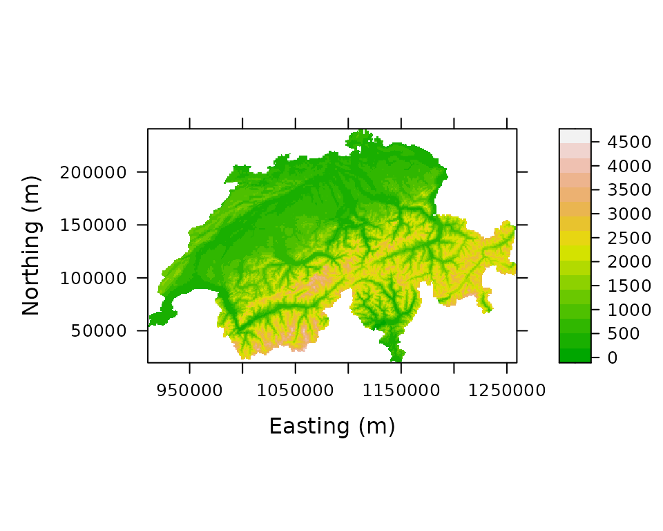

Figure 1. Elevation in Switzerland

The raster package (Jacob van Etten 2012) provides another alternative. Here we create two raster objects and specify the coordinate system.

library(raster)

elevation <- rasterFromXYZ(Switzerland[,c("x","y","elevation")],
    crs="+proj=somerc +lat_0=46.95240555555556 +lon_0=7.439583333333333 +k_0=1 +x_0=600000 +y_0=200000 +ellps=bessel +towgs84=674.374,15.056,405.346,0,0,0,0 +units=m +no_defs")

forest <- rasterFromXYZ(Switzerland[,c("x","y","forest")],
    crs="+proj=somerc +lat_0=46.95240555555556 +lon_0=7.439583333333333 +k_0=1 +x_0=600000 +y_0=200000 +ellps=bessel +towgs84=674.374,15.056,405.346,0,0,0,0 +units=m +no_defs")

Since we standardized the covariates during the model fitting process, we need to transform the country-wide data using the same values. Note, we don’t want to use the mean and SD of the rasters themselves, we want to use the mean and SD of the original covariates used to fit the models, which are stored as attributes of the sc object. The following commands display the original means and SDs and then transform the rasters and join them in a raster “stack”.

attr(sc, "scaled:center")

##        ele     forest 
## 1189.32584   34.74532

attr(sc, "scaled:scale")

##       ele    forest 
## 640.71471  27.67431

ele.s <- (elevation-1189)/640
forest.s <- (forest-34.7)/27.7
ef <- stack(ele.s, forest.s)
names(ef) <- c("ele", "forest")
plot(ef, col=terrain.colors(100))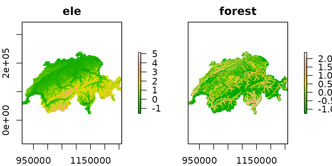

Figure 2. Elevation and forest cover, standardized

It is important to assign names that exactly match the covariate names used to fit the model. This is required by the predict function as demonstrated later. The predict function is useful for computing spatially-referenced model predictions, standard errors, and confidence intervals, but it is computationally demanding when there are many pixels in the raster. Thus, if measures of uncertainty are not required, the following code can be used to quickly produce the species distribution map shown in Fig. 3.

(beta <- coef(fm.occu, type="state"))

##      psi(Int)      psi(ele) psi(I(ele^2))   psi(forest) 
##     0.4638233     1.2276426    -1.3327186     0.6544976

logit.psi <- beta[1] + beta[2]*ele.s + beta[3]*ele.s^2 + beta[4]*forest.s
psi <- exp(logit.psi) / (1 + exp(logit.psi))
print(spplot(psi, col.regions=terrain.colors(100)))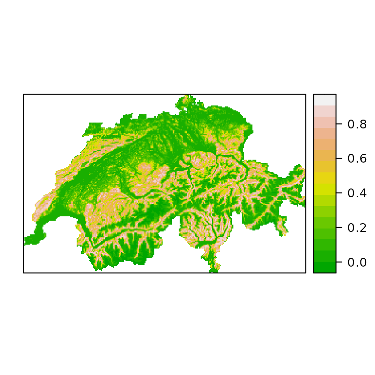

Figure 3. A species distribution map for the European crossbill in Switzerland. The colors represent occurrence probability.

As of version 0.9-6, the predict method in unmarked can make predictions using an object of class RasterStack from the package. As mentioned previously, the rasters must be named, perhaps by using the names(someraster) <- somename method. The object returned by predict is another raster stack with rasters for the expected values of the parameter of interest, the standard errors, and the upper and lower confidence intervals. The following example is very slow because there are many of pixels in the raster. The resulting map is shown in Fig. 4.

E.psi <- predict(fm.occu, type="state", newdata=ef)
plot(E.psi, axes=FALSE, col=terrain.colors(100))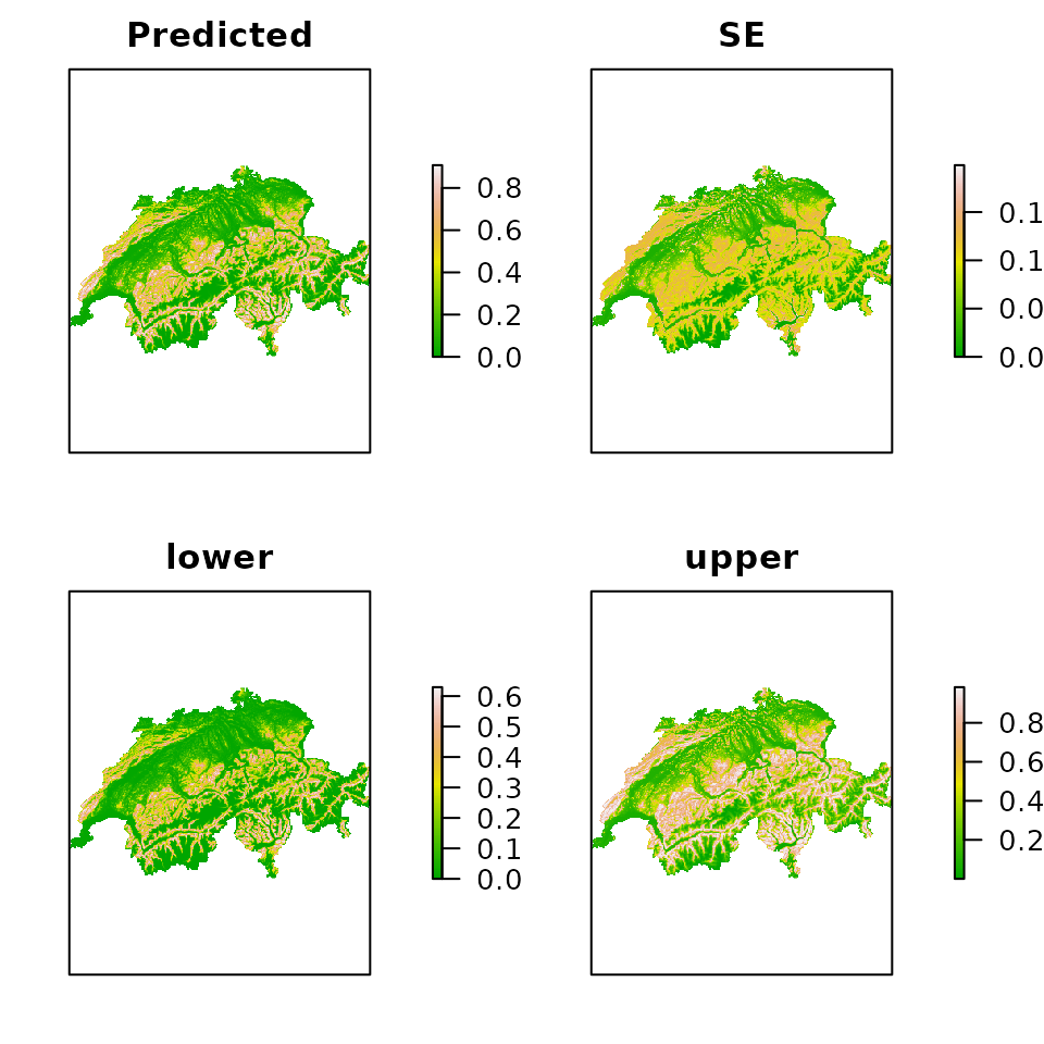

Figure 4. Expected occurrence probability along with standard errors and the limits of the asymptotic 95% confidence interval.

Users should be cautious when predicting from models that have categorical predictor variables, i.e. factors. The package does not have advanced methods for handling factors, and thus it is not easy to automatically create dummy variables from them as can typically be done using model.matrix. The safest option is to create the dummy variables manually before fitting the models, and to use the same variables as rasters for prediction.

A more important consideration when creating species distribution maps based upon occurrence probability is that of spatial scale. Occurrence probability will typically depend upon the area of the “site” in question. Thus, in our crossbill example, it would not be appropriate to use our model to predict occurrence probability for 10-km$^2$ pixels since the surveys were done in 1-km$^2$ quadrats. In some cases it might be possible to directly model the effect of site area on occurrence probability, in which case the effect could be accounted for in the predictions.

Mapping Population Density

Although distribution is typically described in terms of occurrence probability, which is always better than an index of occurrence probability, the best parameter for modeling species distribution is population density because density allows for inference about population size in any region of the species’ range. Furthermore, occurrence probability is simply the probability that abundance is greater than 0, so with density/abundance estimates, it is always possible to compute occurrence probability as a derived parameter.

In this example, we create a distribution map for the Island Scrub-Jay (Aphelocoma insularis), which is restricted to Santa Cruz Island, California. To do so, we fit the hierarchical distance sampling model of Royle et al. (2004), which allows for the estimation of abundance in each of the $300 \times 300$m pixels representing the island. The data were collected 307, 300-m radius point count (or “point transect”) surveyed during the Fall of 2008.

IMPORTANT: This analysis is for demonstration purposes only, and the estimates of population size should not be used for conservation or management purposes. Indeed, the Poisson assumption used here was found to be inadequate by Sillett et al. (2012) who conducted a rigorous analysis and reported reliable estimate of population size.

Although we are fitting a model of population density, the steps of the analysis closely mirror those shown in the previous section. First, we format the data and fit a model, then we format the island-wide covariates and make predictions. The three covariates thought to influence jay abundance are elevation, forest cover, and chapararral cover. We also include include the area of the survey plots in the analysis so that we can make predictions for regions of any area. Here is the code to format the data and fit the model.

data(issj)
covs <- scale(issj[,c("elevation", "forest", "chaparral")])
area <- pi*300^2 / 10000
jayumf <- unmarkedFrameDS(y=as.matrix(issj[,1:3]),
                          siteCovs=data.frame(covs, area),
                          dist.breaks=c(0,100,200,300),
                          unitsIn="m", survey="point")
head(jayumf)

## Data frame representation of unmarkedFrame object.
##    y.1 y.2 y.3   elevation     forest  chaparral     area
## 1    0   0   2 -1.20607849 -0.3309618 -0.1218243 28.27433
## 2    0   0   0 -0.36132054 -0.4429552  0.8384709 28.27433
## 3    0   0   0 -0.45797193 -0.3738751  2.1319298 28.27433
## 4    0   0   0 -0.14196112  1.3908065 -0.2737078 28.27433
## 5    0   0   0 -0.72588125 -0.4869152 -1.1562240 28.27433
## 6    0   0   0  0.01704522  0.6706992  0.2989173 28.27433
## 7    0   0   0 -0.11866710 -0.2671150  1.0326122 28.27433
## 8    0   0   0 -0.76411740 -0.4921486 -0.9332983 28.27433
## 9    0   0   0  0.40065595  0.5440524 -1.0759952 28.27433
## 10   0   0   0 -0.24030211 -0.4921486 -1.1023299 28.27433

fm1 <- distsamp(~chaparral ~chaparral + elevation + offset(log(area)),
                jayumf, keyfun="halfnorm", output="abund",
                starts=c(-2.8,1,0,4.5,0))
fm1

## 
## Call:
## distsamp(formula = ~chaparral ~ chaparral + elevation + offset(log(area)), 
##     data = jayumf, keyfun = "halfnorm", output = "abund", starts = c(-2.8, 
##         1, 0, 4.5, 0))
## 
## Abundance:
##             Estimate     SE      z  P(>|z|)
## (Intercept)   -2.827 0.1609 -17.57 4.34e-69
## chaparral      0.957 0.1460   6.55 5.60e-11
## elevation     -0.244 0.0932  -2.61 8.96e-03
## 
## Detection:
##             Estimate     SE     z  P(>|z|)
## (Intercept)     4.73 0.0845 55.96 0.000000
## chaparral      -0.25 0.0744 -3.36 0.000773
## 
## AIC: 964.6426

Remarks. 1) The distance data were binned into 3 distance classes. 2) We used output="abund" even though, by specifying the offset, we effectively modeled population density. As stated previously, this allows us to make predictions of abundance for regions of arbitrary size.

The next thing to do is to format the raster data. For details, see the previous section-the process is the same, except that we need a raster for "area", the size of each pixel in the raster data. This is necessary because the survey plots were larger than the pixels for which we want predictions of abundance.

data(cruz)
elev <- rasterFromXYZ(cruz[,c("x","y","elevation")],
     crs="+proj=utm +zone=11 +ellps=GRS80 +datum=NAD83 +units=m +no_defs")
forest <- rasterFromXYZ(cruz[,c("x","y","forest")],
     crs="+proj=utm +zone=11 +ellps=GRS80 +datum=NAD83 +units=m +no_defs")
chap <- rasterFromXYZ(cruz[,c("x","y","chaparral")],
     crs="+proj=utm +zone=11 +ellps=GRS80 +datum=NAD83 +units=m +no_defs")
area.raster <- chap
values(area.raster) <- 300*300/10000 # area of a grid pixel
attr(covs, "scaled:center")

##   elevation      forest   chaparral 
## 202.0023616   0.0673357   0.2703592

attr(covs, "scaled:scale")

##   elevation      forest   chaparral 
## 124.8818069   0.1368199   0.2338295

elev.s <- (elev-202)/125
forest.s <- (forest-0.0673)/0.137
chap.s <- (chap-0.270)/0.234
habitat <- stack(elev.s, forest.s, chap.s, area.raster)
names(habitat) <- c("elevation", "forest", "chaparral", "area")

Now, when we use predict, it will return the expected number of jays in each pixel along with the standard errors and the 95% confidence intervals. We could sum these up to obtain an estimate of total population size. Sillett et al. (2012) did this and used the parametric bootstrap to estimate the variance of total population size.

E <- predict(fm1, type="state", newdata=habitat)
plot(E, axes=FALSE, col=terrain.colors(100))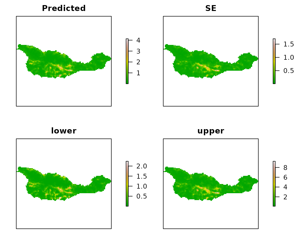

Figure 5. Expeted Island Scrub-Jay abundance, SEs, and 95% CIs.

References

Jacob van Etten, R. J. H. &. 2012. Raster: Geographic analysis and modeling with raster data.

MacKenzie, D. I., J. D. Nichols, G. B. Lachman, S. Droege, J. A. Royle, and C. A. Langtimm. 2002. Estimating site occupancy rates when detection probabilities are less than one. Ecology 83:2248–2255.

Royle, J. A., D. K. Dawson, and S. Bates. 2004. Modeling abundance effects in distance sampling. Ecology 85:1591–1597.

Sarkar, D. 2008. Lattice: Multivariate data visualization with r. Springer, New York.

Schmid, H., N. Zbinden, and V. Keller. 2004. Überwachung der bestandsentwicklung häufiger brutvögel in der schweiz. Swiss Ornithological Institute Sempach Switzerland.

Sillett, S., R. B. Chandler, J. A. Royle, M. Kéry, and S. A. Morrison. 2012. Hierarchical distance sampling models to estimate population size and habitat-specific abundance of an island endemic. Ecological Applications 22:1997–2006.