Community occupancy models with occuComm
Ken Kellner
October 25, 2024
Source:vignettes/occuComm.Rmd
occuComm.RmdIntroduction
In a community occupancy model, detection-nondetection data from multiple species are analyzed together. Intercepts and slopes in the model are species-specific and come from common distributions, allowing for information sharing across species. This structure also allows estimation of site richness. For example, suppose you have sites indexed , occasions and species . The true occupancy state at a site is
with detection data modeled as
Occupancy probability can be modeled as a function of covariates with species-specific random intercepts and slopes coming from common distributions:
A similar structure can be implemented for detection probability .
Note there is a variety of this model that incorporates hypothetical
completely unobserved species using data augmentation, but that is not a
model that unmarked is able to fit at this time.
Example dataset
We’ll use an avian point count dataset from the Swiss breeding bird
survey (MHB) in 2014. The data are counts of 158 species at 267 sites.
The dataset is included in the AHMbook package. For more
detailed analyses of this dataset, see Applied
Hiearchical Modeling in Ecology, Volume 1, section 11.6. You can
also check ?MHB2014 for more information.
## [1] "species" "sites" "counts" "date" "dur"Included in this dataset:
-
species: Species-level information and covariates -
sites: Site covariates -
counts: Counts by site and species -
date: Sampling dates (site by occasion) -
dur: Sampling duration (site by occasion)
Organize the dataset
Detection-nondetection data
We’ll start by converting the count data to detection-nondetection
data (y). The counts are provided in an array format. For
use with occuComm, the y array should have
dimensions site (M) x occasion (J) x species (S). You can also specify
y as a list with length equal to S, with each list element
a matrix with dimensions M x J (similar to occuMulti).
We’ll keep things as an array.
y <- MHB2014$counts
dim(y)
## [1] 267 3 158
y[y > 0] <- 1Species covariates
The model allows for species-level covariates. The covariates must be provided as a named list. Each list element is a separate covariate and can have one of three dimensions: either a vector of length S, a matrix M x S, or an array M x J x S depending on how the covariate varies. For example, you could provide the mean body weight of the species as a vector of length S, or the density of the preferred prey of the species at each site (which could differ by species) as a matrix M x S. In the MHB data, all the species covariates are body size measurements and thus are vectors of length S.
## List of 3
##  $ body.length: int [1:158] 27 48 90 35 102 150 80 58 62 55 ...
##  $ body.mass  : int [1:158] 150 1000 1800 150 3250 11000 3300 1100 1300 1350 ...
##  $ wing.span  : int [1:158] 43 87 165 55 200 220 165 89 91 130 ...
Site covariates
These are organized as usual for unmarked models and are
contained in MHB2014$sites.
##   elev rlength forest
## 1  450     6.4      3
## 2  450     5.5     21
## 3 1050     4.3     32
## 4  950     4.5      9
## 5 1150     5.4     35
## 6  550     3.6      2
Observation covariates
Again these are organized as usual for unmarked (as a
named list).
## $date
##      date141 date142 date143
## Q001      21      52      70
## Q002      26      47      59
## Q003      25      52      73
## Q004      40      55      65
## Q005      16      38      62
## Q006      52      61      69
##
## $dur
##      dur141 dur142 dur143
## Q001    215    220    240
## Q002    195    175    185
## Q003    210    270    210
## Q004    310    300    285
## Q005    240    240    210
## Q006    180    145    140
Create unmarkedFrame
The unmarkedFrame type for this model is called
unmarkedFrameOccuComm. Note the speciesCovs
argument which is unique to this unmarkedFrame type.
library(unmarked)
umf <- unmarkedFrameOccuComm(y = y, siteCovs = sitecov,
                             obsCovs = obscov, speciesCovs = spcov)
head(umf)
## Data frame representation of unmarkedFrame object.
## Only showing observation matrix for species 1.
## y.1 y.2 y.3 elev rlength forest date.1 date.2 date.3 dur.1 dur.2 dur.3
## Q001 0 0 0 450 6.4 3 21 52 70 215 220 240
## Q002 0 0 0 450 5.5 21 26 47 59 195 175 185
## Q003 0 0 0 1050 4.3 32 25 52 73 210 270 210
## Q004 0 0 0 950 4.5 9 40 55 65 310 300 285
## Q005 0 0 0 1150 5.4 35 16 38 62 240 240 210
## Q006 0 0 0 550 3.6 2 52 61 69 180 145 140
## Q007 0 0 0 750 3.9 6 18 40 60 180 195 180
## Q008 0 0 0 650 6.1 60 17 39 61 195 225 210
## Q009 0 0 0 550 5.8 5 18 45 59 190 180 205
## Q010 0 0 0 550 4.5 13 25 50 76 195 203 215Fit a model
With the dataset organized we can now fit a model with
occuComm. We’ll specify a model with an effect of elevation
(site-level) and body mass (species-level) on occupancy, and no
covariates on detection. The occuComm function
automatically sets up the species-level random effects for intercepts
and slopes. Note however that there will be no random slope by species
for species-level covariates of length S (as this would not make sense).
We can specify the model formulas exactly the same as with the
single-species occu function. This model takes a while to
fit given the large number of species.
## Warning: 158 sites have been discarded because of missing data.
fit##
## Call:
## occuComm(formula = ~1 ~ scale(elev) + scale(body.mass), data = umf)
##
## Occupancy (logit-scale):
## Random effects:
## Groups Name Variance Std.Dev.
## species (Intercept) 9.245 3.041
## species scale(elev) 3.169 1.780
##
## Fixed effects:
## Estimate SE z P(>|z|)
## (Intercept) -2.980 0.258 -11.57 5.61e-31
## scale(elev) -0.717 0.155 -4.63 3.64e-06
## scale(body.mass) -0.769 0.272 -2.83 4.72e-03
##
## Detection (logit-scale):
## Random effects:
## Groups Name Variance Std.Dev.
## species (Intercept) 1.663 1.289
##
## Fixed effects:
## Estimate SE z P(>|z|)
## 0.633 0.122 5.19 2.15e-07
##
## AIC: 46368.93
## Number of species: 158
## Number of sites: 266
## ID of sites removed due to NA: 30We get estimates of the overall (mean) intercepts and slopes. We also get estimates of the random effects SDs for the intercepts and for the elevation slopes (but not for body mass, as noted above).
There is some missing data in the model which generates a warning. You can ignore the exact number of missing sites reported by the warning - in fact there is only one missing site (#30) which is reported correctly in the summary.
Estimates of random intercepts and slopes
We can get estimates of the random intercept and slope terms with
randomTerms.
rand_est <- randomTerms(fit)
head(rand_est)
## Model Groups Name Level Estimate SE lower
## 1 psi species (Intercept) Little Grebe -2.659992 1.106212 -4.828127
## 2 psi species (Intercept) Great Crested Grebe -2.359038 1.241233 -4.791811
## 3 psi species (Intercept) Grey Heron -1.517640 1.168330 -3.807526
## 4 psi species (Intercept) Little Bittern -3.668043 1.461535 -6.532599
## 5 psi species (Intercept) White Stork -1.106583 1.439474 -3.927901
## 6 psi species (Intercept) Mute Swan 2.836215 2.545419 -2.152715
## upper
## 1 -0.49185740
## 2 0.07373509
## 3 0.77224458
## 4 -0.80348815
## 5 1.71473497
## 6 7.82514579
tail(rand_est)## Model Groups Name Level Estimate SE
## 469 p species (Intercept) Corn Bunting -1.04598590 1.0409023
## 470 p species (Intercept) Yellowhammer 1.49688629 0.2277654
## 471 p species (Intercept) Cirl Bunting -0.71401947 0.5916209
## 472 p species (Intercept) Ortolan Bunting -0.07100565 1.3653792
## 473 p species (Intercept) Rock Bunting 0.40225149 0.2812063
## 474 p species (Intercept) Common Reed Bunting -0.44832431 0.6252049
## lower upper
## 469 -3.0861169 0.9941451
## 470 1.0504743 1.9432983
## 471 -1.8735751 0.4455361
## 472 -2.7470997 2.6050885
## 473 -0.1489027 0.9534057
## 474 -1.6737033 0.7770547The estimates provided by this function are mean-0 (i.e., they come
from a normal distribution with mean 0). Thus to get the complete
intercept and slope for each species, we need to add the “fixed” part of
the intercept and slope (shown in the Fixed effects section
of the summary, or with coef()) to the random part shown
above. We can do this with an argument:
rand_est <- randomTerms(fit, addMean = TRUE)
head(rand_est)
## Model Groups Name Level Estimate SE lower
## 1 psi species (Intercept) Little Grebe -5.6402732 1.088450 -7.773597
## 2 psi species (Intercept) Great Crested Grebe -5.3393185 1.226390 -7.742998
## 3 psi species (Intercept) Grey Heron -4.4979213 1.147969 -6.747900
## 4 psi species (Intercept) Little Bittern -6.6483243 1.452614 -9.495396
## 5 psi species (Intercept) White Stork -4.0868639 1.422657 -6.875221
## 6 psi species (Intercept) Mute Swan -0.1440654 2.533089 -5.108828
## upper
## 1 -3.506950
## 2 -2.935639
## 3 -2.247943
## 4 -3.801252
## 5 -1.298507
## 6 4.820697Get estimates of occupancy
As usual with unmarked, we can use predict.
The predict function will return estimates of occupancy for
each site and species by default.
## $`Little Grebe`
## Predicted SE lower upper
## 1 0.062629441 0.027968118 0.025591420 0.14527977
## 2 0.062629441 0.027968118 0.025591420 0.14527977
## 3 0.006932087 0.006147293 0.001211306 0.03862620
## 4 0.010069015 0.007592241 0.002280547 0.04330204
## 5 0.004767739 0.004893379 0.000634300 0.03489633
## 6 0.043842917 0.018741413 0.018733213 0.09920657
##
## $`Great Crested Grebe`
## Predicted SE lower upper
## 1 0.040469236 0.023611754 0.0126461928 0.12194572
## 2 0.040469236 0.023611754 0.0126461928 0.12194572
## 3 0.004956348 0.004995188 0.0006837188 0.03499409
## 4 0.007061007 0.006133672 0.0012785527 0.03800045
## 5 0.003476823 0.004020987 0.0003586577 0.03281439
## 6 0.028694428 0.015960275 0.0095246153 0.08320543
##
## $`Grey Heron`
## Predicted SE lower upper
## 1 0.047915787 0.024412407 0.0173265386 0.12560618
## 2 0.047915787 0.024412407 0.0173265386 0.12560618
## 3 0.006356595 0.005769278 0.0010666779 0.03691114
## 4 0.008941182 0.006947514 0.0019367894 0.04025524
## 5 0.004515718 0.004725964 0.0005775214 0.03438506
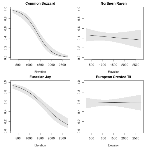
## 6 0.034456683 0.016614842 0.0132319646 0.08673438Plot covariate relationships by species
We’ll plot estimated occupancy by elevation for four species: Common Buzzard, Northern Raven, Eurasian Jay, and European Crested Tit. We also need to get the corresponding body mass of each species.
sp <- c("Common Buzzard", "Northern Raven", "Eurasian Jay", "European Crested Tit")
body_mass <- MHB2014$species$body.mass
names(body_mass) <- MHB2014$species$engname
body_mass <- unname(body_mass[sp])
First create a sequence of elevation values.
For each species we create a newdata data frame with
elevation and the species name and matching body mass. Then we use
predict, and plot the results.
par(mfrow=c(2,2), mar=c(4,3,2,1))
for (i in 1:length(sp)){
  nd <- data.frame(elev=elev_seq,
                   species = sp[i],
                   body.mass = body_mass[i])
  pr <- predict(fit, 'state', newdata=nd)
  plot(elev_seq, pr$Predicted, type='l', xlab="Elevation", ylab="Occupancy",
       main = sp[i], ylim=c(0,1))
  polygon(c(elev_seq, rev(elev_seq)), c(pr$lower, rev(pr$upper)), col='grey90', border=NA)
  lines(elev_seq, pr$Predicted)
}
Richness
There’s a built-in function for calculating richness at each site from the model.
## [1] 33.49 34.93 52.52 42.07 45.55 43.46To get the uncertainty of this estimate, we can return a complete posterior and calculate CIs:
post <- richness(fit, posterior=TRUE)
est <- apply(post@samples, 1, mean)
low <- apply(post@samples, 1, quantile, 0.025)
up <- apply(post@samples, 1, quantile, 0.975)
And compare them to naive richness:
rich_naive <- MHB2014$counts
rich_naive[rich_naive > 0] <- 1
rich_naive <- apply(rich_naive, c(1,3),
                    function(x) if(all(is.na(x))) return(NA) else return(max(x, na.rm=TRUE)))
rich_naive <- apply(rich_naive, 1, sum, na.rm=TRUE)

plot(rich_naive, est, xlab="Observed species", ylab="Estimated richness",
     pch=19, col=rgb(0,0,0,alpha=0.2))
segments(rich_naive, low, rich_naive, up)
abline(a=0, b=1)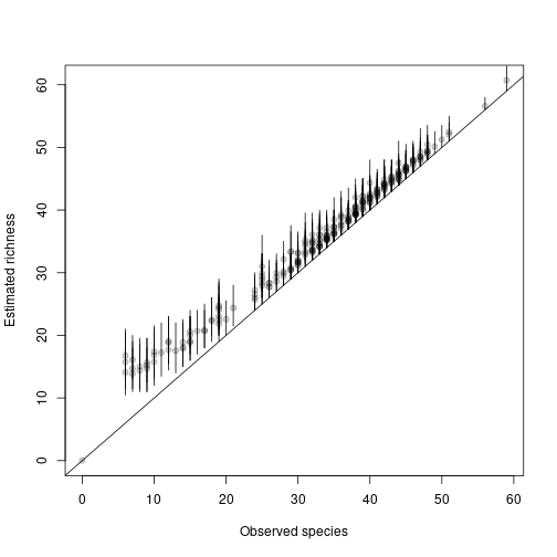
This figure should look similar to Figure 11.8 in the AHM 1 book (it’s not quite the same model).
Handling guilds or similar groups
In community occupancy models it is common to specify an additional hierarchical structure above species, e.g. guild. In this version of the model, rather than the random intercepts and slopes coming from common distributions across all species, instead information is shared only among species belonging to the same guild. The model structure is the same as above except the random effect hyperparameters are guild-specific where each species belongs to one guild .
For example, see the analysis in section 11.6.3 of AHM 1.
The occuComm function cannot directly handle this extra
hierarchical layer as you can in say, JAGS or NIMBLE. However, we can
get pretty close. Note that often when we fit a guild-based model like
this, we are in effect fitting entirely separate models for each guild.
That is, since no information is being shared among guilds (only within
them) we can simply separate the data by guild and fit separate models
to each piece and get the same result. We can then combine the results
to get richness, if needed. This occuComm is able to
do.
Dividing the data by guild
We’ll divide the species into three “guilds” based on body mass. This code is identical to the code in AHM 1, section 11.6.3.
# Look at distribution of body mass among 136 observed species
# Get mean species mass
mass <- MHB2014$species$body.mass
hist(log10(mass), breaks = 40, col = "grey")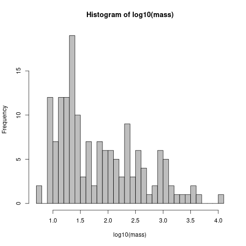
# Look at log10
gmass <- as.numeric(log10(mass) %/% 1.3 + 1)
# Size groups 1, 2 and 3
gmass[gmass == 4] <- 3 # Mute swan is group 3, too
Fit separate models by guild
Now we simply divide our complete dataset into pieces by guild and fit the same model to each dataset separately.
# Guild 1
spcovs1 <- lapply(spcov, function(x) x[gmass == 1])
umf1 <- unmarkedFrameOccuComm(y = umf@ylist[gmass == 1],
                              siteCovs = sitecov,
                              obsCovs = obscov,
                              speciesCovs = spcovs1)
fit1 <- update(fit, data = umf1)
## Warning: 45 sites have been discarded because of missing data.
# Guild 2
spcovs2 <- lapply(spcov, function(x) x[gmass == 2])
umf2 <- unmarkedFrameOccuComm(y = umf@ylist[gmass == 2],
                              siteCovs = sitecov,
                              obsCovs = obscov,
                              speciesCovs = spcovs2)
fit2 <- update(fit, data = umf2)
## Warning: 86 sites have been discarded because of missing data.
# Guild 3
spcovs3 <- lapply(spcov, function(x) x[gmass == 3])
umf3 <- unmarkedFrameOccuComm(y = umf@ylist[gmass == 3],
                              siteCovs = sitecov,
                              obsCovs = obscov,
                              speciesCovs = spcovs3)
fit3 <- update(fit, data = umf3)
## Warning: 27 sites have been discarded because of missing data.Calculate richness
To get richness across the entire community, we get posterior samples of richness for each guild and combine them.
post1 <- richness(fit1, posterior=TRUE)
post2 <- richness(fit2, posterior=TRUE)
post3 <- richness(fit3, posterior=TRUE)
rich_all <- post1@samples + post2@samples + post3@samples
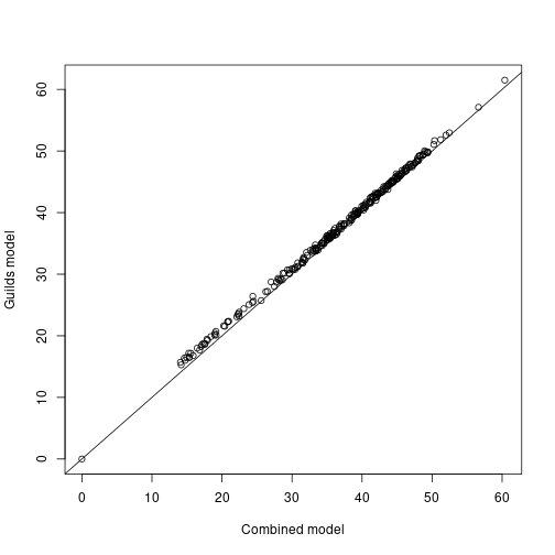
rich_all <- drop(rich_all)The result is more or less identical to our previous richness estimate using a single model.
rich_mean <- apply(rich_all, 1, mean)
plot(rich, rich_mean, xlab="Combined model", ylab="Guilds model")
abline(a=0, b=1)