Generalized multinomial N-mixture model

A three level hierarchical model for designs involving repeated counts that yield multinomial outcomes. Possible data collection methods include repeated removal sampling and double observer sampling. The three model parameters are abundance, availability, and detection probability.

gmultmix(lambdaformula, phiformula, pformula, data, mixture = c("P", "NB", "ZIP"), K, 
         starts, method = "BFGS", se = TRUE, engine=c("C","R"), threads=1, ...)

Arguments

lambdaformula: Righthand side (RHS) formula describing abundance covariates
phiformula: RHS formula describing availability covariates
pformula: RHS formula describing detection covariates
data: An object of class unmarkedFrameGMM
mixture: Either "P", "NB", or "ZIP" for the Poisson, negative binomial, or zero-inflated Poisson models of abundance
K: The upper bound of integration
starts: Starting values
method: Optimization method used by optim
se: Logical. Should standard errors be calculated?
engine: Either "C" to use fast C++ code or "R" to use native R code during the optimization.
threads: Set the number of threads to use for optimization in C++, if OpenMP is available on your system. Increasing the number of threads may speed up optimization in some cases by running the likelihood calculation in parallel. If threads=1 (the default), OpenMP is disabled.
...: Additional arguments to optim, such as lower and upper bounds

Details

The latent transect-level super-population abundance distribution \(f(M | \mathbf{\theta})\) can be set as a Poisson, negative binomial, or zero-inflated Poisson random variable, depending on the setting of the mixture argument. mixture = "P", mixture = "NB", and mixture = "ZIP" select the Poisson, negative binomial, and zero-inflated Poisson distributions respectively. The mean of \(M_i\) is \(\lambda_i\). If \(M_i \sim NB\), then an additional parameter, \(\alpha\), describes dispersion (lower \(\alpha\) implies higher variance). If \(M_i \sim ZIP\), then an additional zero-inflation parameter \(\psi\) is estimated.

The number of individuals available for detection at time j is a modeled as binomial: \(N_{ij} \sim Binomial(M_i, \mathbf{\phi_{ij}})\).

The detection process is modeled as multinomial: \(\mathbf{y_{it}} \sim Multinomial(N_{it}, \pi_{it})\), where \(\pi_{ijt}\) is the multinomial cell probability for plot i at time t on occasion j.

Cell probabilities are computed via a user-defined function related to the sampling design. Alternatively, the default functions removalPiFun or doublePiFun can be used for equal-interval removal sampling or double observer sampling. Note that the function for computing cell probabilites is specified when setting up the data using unmarkedFrameGMM.

Parameters \(\lambda\), \(\phi\) and \(p\) can be modeled as linear functions of covariates using the log, logit and logit links respectively.

Value

An object of class unmarkedFitGMM.

References

Royle, J. A. (2004) Generalized estimators of avian abundance from count survey data. Animal Biodiversity and Conservation 27, pp. 375–386.

Chandler, R. B., J. A. Royle, and D. I. King. 2011. Inference about density and temporary emigration in unmarked populations. Ecology 92:1429-1435.

Author

Richard Chandler rbchan@uga.edu and Andy Royle

Note

In the case where availability for detection is due to random temporary emigration, population density at time j, D(i,j), can be estimated by N(i,j)/plotArea.

This model is also applicable to sampling designs in which the local population size is closed during the J repeated counts, and availability is related to factors such as the probability of vocalizing. In this case, density can be estimated by M(i)/plotArea.

If availability is a function of both temporary emigration and other processess such as song rate, then density cannot be directly estimated, but inference about the super-population size, M(i), is possible.

Three types of covariates can be supplied, site-level, site-by-year-level, and observation-level. These must be formatted correctly when organizing the data with unmarkedFrameGPC

Examples


# Simulate data using the multinomial-Poisson model with a
# repeated constant-interval removal design.

n <- 100  # number of sites
T <- 4    # number of primary periods
J <- 3    # number of secondary periods

lam <- 3
phi <- 0.5
p <- 0.3

#set.seed(26)
y <- array(NA, c(n, T, J))
M <- rpois(n, lam)          # Local population size
N <- matrix(NA, n, T)       # Individuals available for detection

for(i in 1:n) {
    N[i,] <- rbinom(T, M[i], phi)
    y[i,,1] <- rbinom(T, N[i,], p)    # Observe some
    Nleft1 <- N[i,] - y[i,,1]         # Remove them
    y[i,,2] <- rbinom(T, Nleft1, p)   # ...
    Nleft2 <- Nleft1 - y[i,,2]
    y[i,,3] <- rbinom(T, Nleft2, p)
    }

y.ijt <- cbind(y[,1,], y[,2,], y[,3,], y[,4,])


umf1 <- unmarkedFrameGMM(y=y.ijt, numPrimary=T, type="removal")

(m1 <- gmultmix(~1, ~1, ~1, data=umf1, K=30))
#> 
#> Call:
#> gmultmix(lambdaformula = ~1, phiformula = ~1, pformula = ~1, 
#>     data = umf1, K = 30)
#> 
#> Abundance:
#>  Estimate    SE    z  P(>|z|)
#>     0.943 0.135 6.99 2.71e-12
#> 
#> Availability:
#>  Estimate    SE     z P(>|z|)
#>     0.422 0.464 0.909   0.364
#> 
#> Detection:
#>  Estimate    SE     z  P(>|z|)
#>     -1.05 0.251 -4.17 3.04e-05
#> 
#> AIC: 1538.859 

backTransform(m1, type="lambda")        # Individuals per plot
#> Backtransformed linear combination(s) of Abundance estimate(s)
#> 
#>  Estimate    SE LinComb (Intercept)
#>      2.57 0.346   0.943           1
#> 
#> Transformation: exp 
backTransform(m1, type="phi")           # Probability of being avilable
#> Backtransformed linear combination(s) of Availability estimate(s)
#> 
#>  Estimate    SE LinComb (Intercept)
#>     0.604 0.111   0.422           1
#> 
#> Transformation: logistic 
(p <- backTransform(m1, type="det"))    # Probability of detection
#> Backtransformed linear combination(s) of Detection estimate(s)
#> 
#>  Estimate     SE LinComb (Intercept)
#>      0.26 0.0482   -1.05           1
#> 
#> Transformation: logistic 
p <- coef(p)

# Multinomial cell probabilities under removal design
c(p, (1-p) * p, (1-p)^2 * p)
#> [1] 0.2600816 0.1924392 0.1423893

# Or more generally:
head(getP(m1))
#>           [,1]      [,2]      [,3]      [,4]      [,5]      [,6]      [,7]
#> [1,] 0.2600816 0.1924392 0.1423893 0.2600816 0.1924392 0.1423893 0.2600816
#> [2,] 0.2600816 0.1924392 0.1423893 0.2600816 0.1924392 0.1423893 0.2600816
#> [3,] 0.2600816 0.1924392 0.1423893 0.2600816 0.1924392 0.1423893 0.2600816
#> [4,] 0.2600816 0.1924392 0.1423893 0.2600816 0.1924392 0.1423893 0.2600816
#> [5,] 0.2600816 0.1924392 0.1423893 0.2600816 0.1924392 0.1423893 0.2600816
#> [6,] 0.2600816 0.1924392 0.1423893 0.2600816 0.1924392 0.1423893 0.2600816
#>           [,8]      [,9]     [,10]     [,11]     [,12]
#> [1,] 0.1924392 0.1423893 0.2600816 0.1924392 0.1423893
#> [2,] 0.1924392 0.1423893 0.2600816 0.1924392 0.1423893
#> [3,] 0.1924392 0.1423893 0.2600816 0.1924392 0.1423893
#> [4,] 0.1924392 0.1423893 0.2600816 0.1924392 0.1423893
#> [5,] 0.1924392 0.1423893 0.2600816 0.1924392 0.1423893
#> [6,] 0.1924392 0.1423893 0.2600816 0.1924392 0.1423893

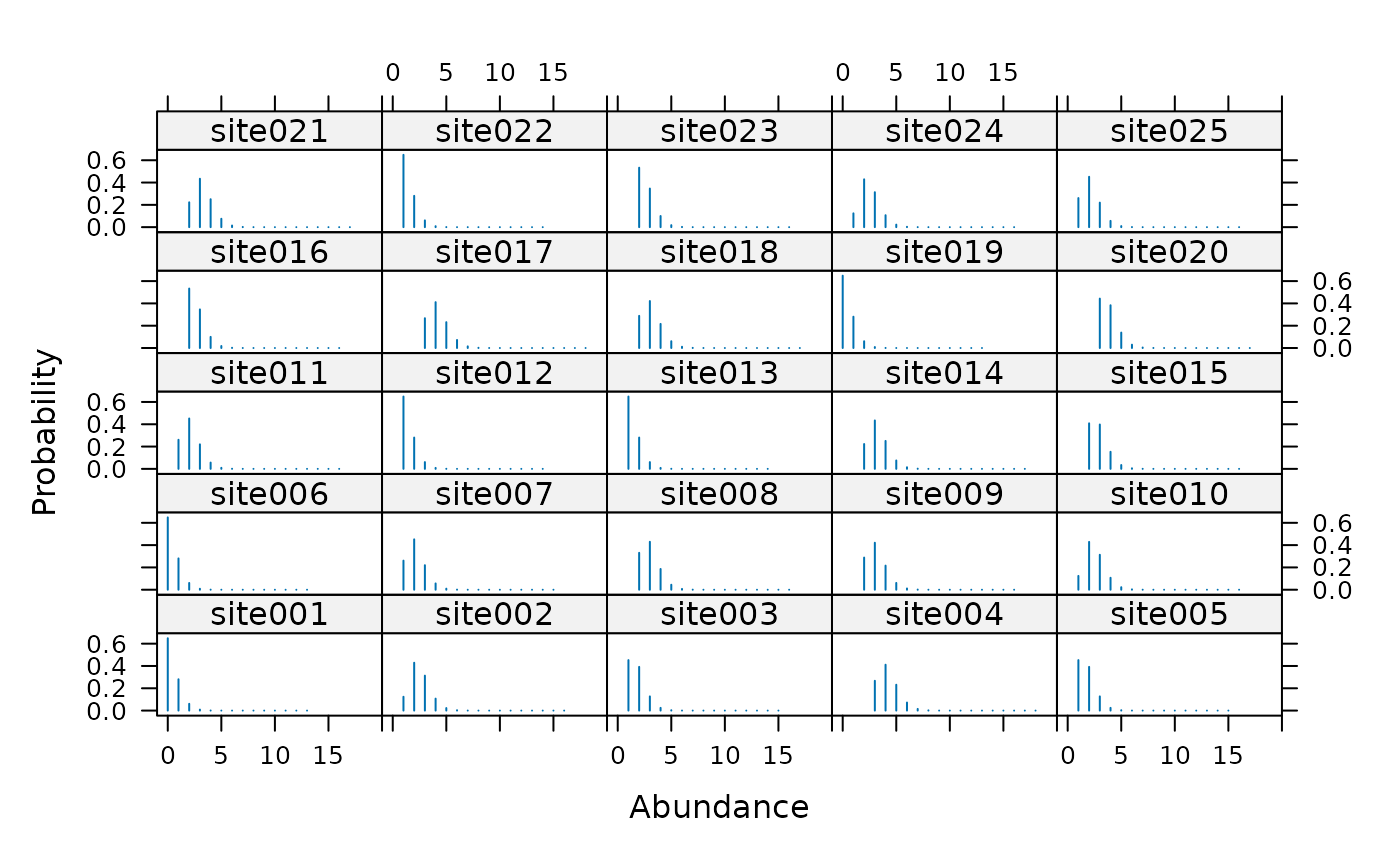
# Empirical Bayes estimates of super-population size
re <- ranef(m1)
plot(re, layout=c(5,5), xlim=c(-1,20), subset=site%in%1:25)